Getting started
Once FluidSF is installed, you can load the module into Python and run some basic calculations with random data.
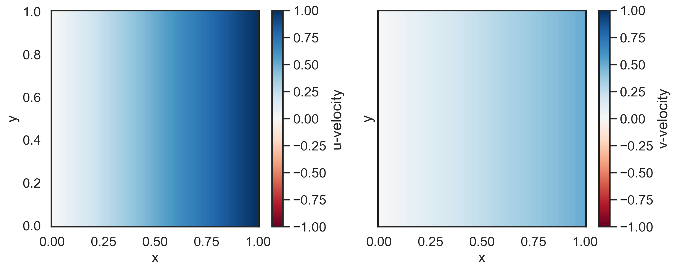
Create a 2D velocity field
We will generate u and v velocity arrays that increase linearly in x. The v velocity will be half the magnitude of the u velocity.
[2]:
import numpy as np

nx, ny = 100, 100
x = np.linspace(0, 1, nx)
y = np.linspace(0, 1, ny)
X, Y = np.meshgrid(x, y)

u = X
v = 0.5 * X
[3]:
import matplotlib.pyplot as plt

fig, (ax1, ax2) = plt.subplots(1, 2, sharex=True, sharey=True, figsize=(12, 5))
p1 = ax1.pcolormesh(x, y, u, cmap="RdBu", vmin=-1, vmax=1)
p2 = ax2.pcolormesh(x, y, v, cmap="RdBu", vmin=-1, vmax=1)
fig.colorbar(p1, label="u-velocity")
fig.colorbar(p2, label="v-velocity")
ax1.set_xlabel("x")
ax2.set_xlabel("x")
ax1.set_ylabel("y")
ax2.set_ylabel("y")
plt.tight_layout()
Generate the velocity structure function
We can generate structure function using the function generate_structure_functions_2d. The function returns a dictionary with the all supported structure functions and separation distances in each direction.
By default the advective velocity structure functions are calculated and the remaining structure functions are set to None. To calculate all velocity structure functions we set sf_type=["ASF_V", "LLL", "LL", "LTT"].
We set the boundary condition to None because our random data is non-periodic. If we had periodic data we could set the boundary condition based on the direction of periodicity (i.e. boundary="periodic-x" or boundary="periodic-y" or boundary="periodic-all" for 2D data).
[4]:
import fluidsf

sf = fluidsf.generate_structure_functions_2d(
    u, v, x, y, sf_type=["ASF_V", "LLL", "LL", "LTT"], boundary=None
)
The keys of the dictionary sf are
SF_advection_velocity_dir: Advective velocity structure function in the direction of the separation vector (dir=x,y,z).SF_advection_scalar_dir: Advective scalar structure function in the direction of the separation vector (dir=x,y,z).SF_LL_dir: Longitudinal second order velocity structure function in the direction of the separation vector (dir=x,y,z).SF_LLL_dir: Longitudinal third order velocity structure function in the direction of the separation vector (dir=x,y,z).SF_LTT_dir: Longitudinal-transverse-transverse third order velocity structure function in the direction of the separation vector (dir=x,y,z).SF_LSS_dir: Longitudinal-scalar-scalar third order velocity structure function in the direction of the separation vector (dir=x,y,z).dir-diffs: Separation distances in each direction (dir=x,y,z).
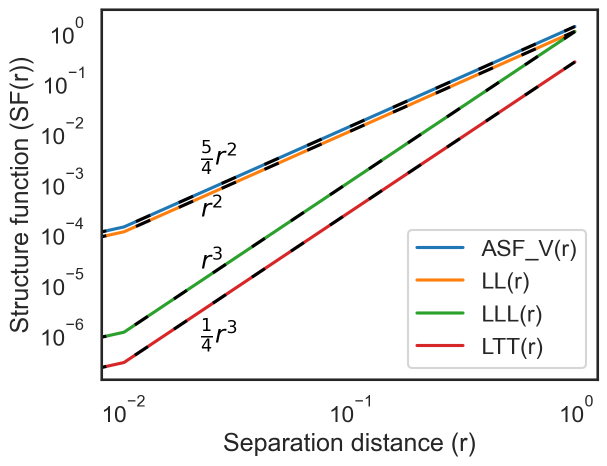
Plot the advective velocity structure functions in x and y
[5]:
fig, ax = plt.subplots()
ax.loglog(sf["x-diffs"], sf["SF_advection_velocity_x"], label="ASF_V(r)", color="C0")
ax.loglog(sf["x-diffs"], sf["SF_LL_x"], label="LL(r)", color="C1")
ax.loglog(sf["x-diffs"], sf["SF_LLL_x"], label="LLL(r)", color="C2")
ax.loglog(sf["x-diffs"], sf["SF_LTT_x"], label="LTT(r)", color="C3")
ax.loglog(
    sf["x-diffs"],
    (5 / 4) * sf["x-diffs"] ** 2,
    color="k",
    linestyle=(0, (5, 10)),
)
ax.loglog(sf["x-diffs"], sf["x-diffs"] ** 2, color="k", linestyle=(0, (5, 10)))
ax.loglog(sf["x-diffs"], sf["x-diffs"] ** 3, color="k", linestyle=(0, (5, 10)))
ax.loglog(
    sf["x-diffs"],
    0.25 * sf["x-diffs"] ** 3,
    color="k",
    linestyle=(0, (5, 10)),
)

ax.annotate(
    r"$\frac{5}{4}r^{2}$",
    (0.2, 0.58),
    textcoords="axes fraction",
    color="k",
)

ax.annotate(
    r"$r^{2}$",
    (0.2, 0.44),
    textcoords="axes fraction",
    color="k",
)

ax.annotate(
    r"$r^{3}$",
    (0.2, 0.3),
    textcoords="axes fraction",
    color="k",
)

ax.annotate(
    r"$\frac{1}{4}r^{3}$",
    (0.2, 0.1),
    textcoords="axes fraction",
    color="k",
)

plt.hlines(0, 0, 1, color="k", lw=1, zorder=0)
ax.set_xlabel("Separation distance (r)")
ax.set_ylabel("Structure function (SF(r))")
ax.legend(loc="lower right")
plt.show()
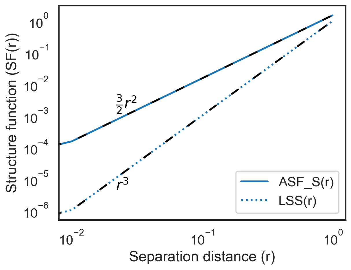
Scalar structure functions
The scalar structure functions can be generated by including "ASF_S" and/or "LSS" in sf_type.
[6]:
S = X + Y

sf = fluidsf.generate_structure_functions_2d(
    u, v, x, y, sf_type=["ASF_S", "LSS"], scalar=S, boundary=None
)
[7]:
import matplotlib.pyplot as plt

fig, ax = plt.subplots()
ax.loglog(
    sf["x-diffs"],
    sf["SF_advection_scalar_x"],
    label="ASF_S(r)",
    color="tab:blue",
)

ax.loglog(
    sf["x-diffs"],
    sf["SF_LSS_x"],
    label="LSS(r)",
    color="tab:blue",
    linestyle="dotted",
)

ax.loglog(
    sf["x-diffs"], (3 / 2) * sf["x-diffs"] ** 2, color="k", linestyle=(0, (5, 10))
)
ax.loglog(sf["x-diffs"], sf["x-diffs"] ** 3, color="k", linestyle=(0, (5, 10)))

ax.annotate(
    r"$\frac{3}{2}r^{2}$",
    (0.2, 0.52),
    textcoords="axes fraction",
    color="k",
)

ax.annotate(
    r"$r^{3}$",
    (0.2, 0.14),
    textcoords="axes fraction",
    color="k",
)

plt.hlines(0, 0, 1, color="k", lw=1, zorder=0)
ax.set_xlabel("Separation distance (r)")
ax.set_ylabel("Structure function (SF(r))")
ax.legend(loc="lower right")
plt.show()