Structure functions with 2D data
This example will guide you through each step necessary to compute velocity- and vorticity-based structure functions from a 2D simulation of surface ocean velocity.
General procedure:
Load a dataset generated with GeophysicalFlows.jl
Format the dataset
Calculate velocity-based and scalar-based structure functions for the zonal and meridional directions as a function of separation distance
Plot the structure functions as a function of separation distance
Download sample dataset with Pooch
We will use Pooch to download a sample dataset.
[2]:
import pooch

file_path = pooch.retrieve(
    url="https://zenodo.org/records/15278227/files/2layer_128.jld2",
    known_hash="a04abc602ca3bbc4ff9a868a96848b6815a17f697202fb12e3ff40762de92ec6")
Load the dataset generated with GeophysicalFlows.jl
We will use h5py to load a .jld2 file, the output from GeophysicalFlows.jl, a numerical ocean simulator written in Julia.
[3]:
import h5py

f = h5py.File(file_path, 'r')
grid = f['grid']
snapshots = f['snapshots']

# Initialize the grid of x and y coordinates
x = grid['x'][()]
y = grid['y'][()]

# Grab the top layer and final snapshot of the simulation for u, v, and q
u = snapshots['u']['20050'][0]
v = snapshots['v']['20050'][0]
q = snapshots['q']['20050'][0]
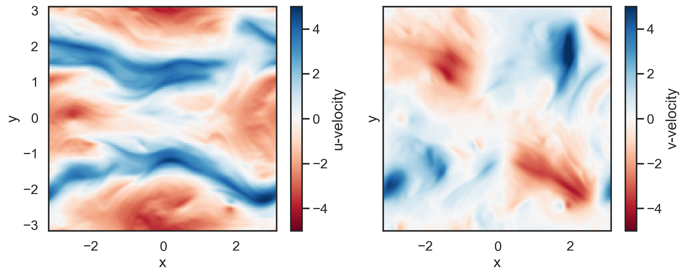
Make a couple of quick plots to see the velocity fields.
[4]:
import matplotlib.pyplot as plt

fig, (ax1, ax2) = plt.subplots(1,2, sharex=True, sharey=True, figsize=(12,5))
p1 = ax1.pcolormesh(x,y,u, cmap='RdBu',vmin=-5,vmax=5)
p2 = ax2.pcolormesh(x,y,v, cmap='RdBu',vmin=-5,vmax=5)
fig.colorbar(p1,label='u-velocity')
fig.colorbar(p2, label='v-velocity')
ax1.set_xlabel('x')
ax2.set_xlabel('x')
ax1.set_ylabel('y')
ax2.set_ylabel('y')
plt.tight_layout()
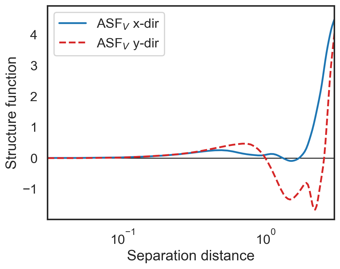
Calculate advective velocity structure functions
By default fluidsf.generate_structure_functions_2d will generate the advective velocity-based structure function.
[5]:
import fluidsf

sf = fluidsf.generate_structure_functions_2d(u, v, x, y)
[6]:
fig, (ax1) = plt.subplots()


ax1.semilogx(sf['x-diffs'], sf['SF_advection_velocity_x'],
             label=r'ASF$_V$ x-dir',color='tab:blue')
ax1.semilogx(sf['y-diffs'], sf['SF_advection_velocity_y'],
             label=r'ASF$_V$ y-dir',
             color='tab:red',linestyle='dashed')

ax1.set_ylabel(r"Structure function")
ax1.set_xlabel(r"Separation distance")
ax1.set_xlim(3e-2,3e0)
ax1.legend()
plt.hlines(0,3e-2,3e0,color='k',lw=1,zorder=0);
Calculating scalar-based structure functions and traditional structure functions
We can repeat the above steps with additional inputs to calculate advective structure functions from scalar fields as well as traditional structure functions.
Note: we now add "ASF_V" to the list given to sf_type because otherwise the advective velocity structure function will be skipped.
[7]:
sf_all = fluidsf.generate_structure_functions_2d(
    u,
    v,
    x,
    y,
    sf_type=["ASF_V", "ASF_S", "LLL", "LL", "LTT", "LSS"],
    scalar=q,
)
[8]:
fig, (ax1) = plt.subplots()


ax1.semilogx(sf_all['x-diffs'], sf_all['SF_advection_scalar_x'],
             label=r'ASF$_{\omega}$ x-dir',
             color='tab:blue')
ax1.semilogx(sf_all['y-diffs'], sf_all['SF_advection_scalar_y'],
             label=r'ASF$_{\omega}$ y-dir',
             color='tab:red', linestyle='dashed')

ax1.set_ylabel(r"Structure function")
ax1.set_xlabel(r"Separation distance")
ax1.set_xlim(3e-2,3e0)
ax1.legend()
plt.hlines(0,3e-2,3e0,color='k',lw=1,zorder=0)
ax1.tick_params(direction="in", which="both")
ax1.xaxis.get_ticklocs(minor=True)
ax1.minorticks_on()
[9]:
fig, (ax1) = plt.subplots()


ax1.semilogx(sf_all['x-diffs'], sf_all['SF_LLL_x'],
             label=r'LLL x-dir',
             color='tab:blue')
ax1.semilogx(sf_all['y-diffs'], sf_all['SF_LLL_y'],
             label=r'LLL y-dir',
             color='tab:red',linestyle='dashed')

ax1.set_ylabel(r"Structure function")
ax1.set_xlabel(r"Separation distance")
ax1.set_xlim(3e-2,3e0)
ax1.legend()
plt.hlines(0,3e-2,3e0,color='k',lw=1,zorder=0)
ax1.tick_params(direction="in", which="both")
ax1.xaxis.get_ticklocs(minor=True)
ax1.minorticks_on()

[10]:
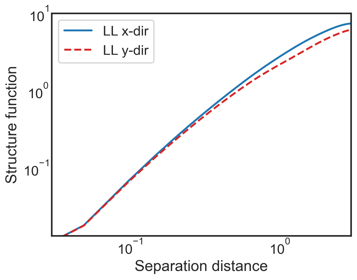
fig, (ax1) = plt.subplots()


ax1.loglog(sf_all['x-diffs'], sf_all['SF_LL_x'],
             label=r'LL x-dir',
             color='tab:blue')
ax1.loglog(sf_all['y-diffs'], sf_all['SF_LL_y'],
             label=r'LL y-dir',
             color='tab:red',linestyle='dashed')

ax1.set_ylabel(r"Structure function")
ax1.set_xlabel(r"Separation distance")
ax1.set_xlim(3e-2,3e0)
ax1.legend()
plt.hlines(0,3e-2,3e0,color='k',lw=1,zorder=0)
ax1.tick_params(direction="in", which="both")
ax1.xaxis.get_ticklocs(minor=True)
ax1.minorticks_on()

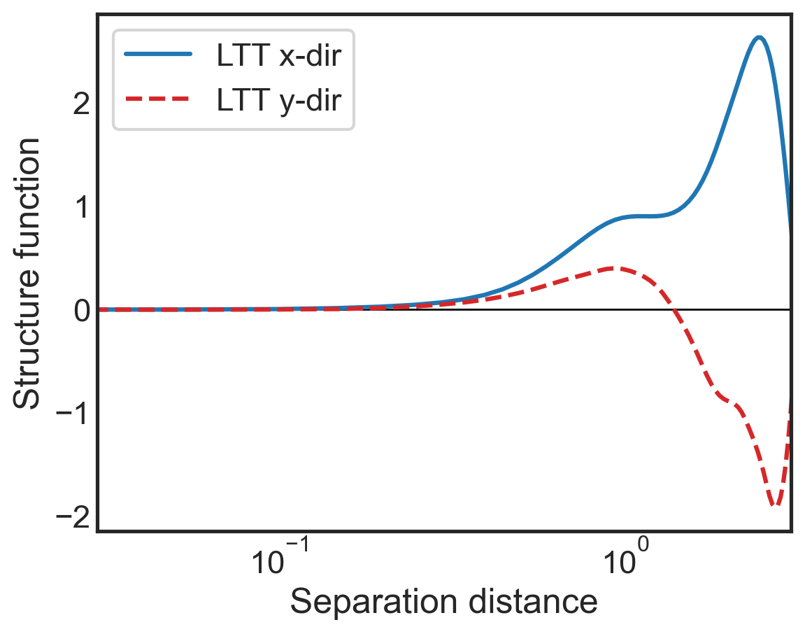
[11]:
fig, (ax1) = plt.subplots()


ax1.semilogx(sf_all['x-diffs'], sf_all['SF_LTT_x'],
             label=r'LTT x-dir',
             color='tab:blue')
ax1.semilogx(sf_all['y-diffs'], sf_all['SF_LTT_y'],
             label=r'LTT y-dir',
             color='tab:red',linestyle='dashed')

ax1.set_ylabel(r"Structure function")
ax1.set_xlabel(r"Separation distance")
ax1.set_xlim(3e-2,3e0)
ax1.legend()
plt.hlines(0,3e-2,3e0,color='k',lw=1,zorder=0)
ax1.tick_params(direction="in", which="both")
ax1.xaxis.get_ticklocs(minor=True)
ax1.minorticks_on()
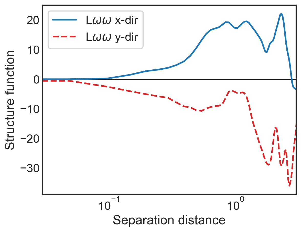
[12]:
fig, (ax1) = plt.subplots()


ax1.semilogx(sf_all['x-diffs'], sf_all['SF_LSS_x'],
             label=r'L$\omega\omega$ x-dir',
             color='tab:blue')
ax1.semilogx(sf_all['y-diffs'], sf_all['SF_LSS_y'],
             label=r'L$\omega\omega$ y-dir',
             color='tab:red', linestyle='dashed')

ax1.set_ylabel(r"Structure function")
ax1.set_xlabel(r"Separation distance")
ax1.set_xlim(3e-2,3e0)
ax1.legend()
plt.hlines(0,3e-2,3e0,color='k',lw=1,zorder=0)
ax1.tick_params(direction="in", which="both")
ax1.xaxis.get_ticklocs(minor=True)
ax1.minorticks_on()