Structure functions with 3D data
This example will walk you through the steps required to generate structure functions for a 3D velocity field. The example data was generated with Oceananigans.jl.
General procedure:
Set up plot environment and load the dataset
Plot the velocity fields and spatial gradients
Calculate a variety of structure functions along different directions
Plot structure functions as a function of length scale
Download sample dataset with Pooch
We will use Pooch to download a sample dataset.
[2]:
import pooch

file_path = pooch.retrieve(
    url="https://zenodo.org/records/15278227/files/langmuir_fields.nc",
    known_hash="d32f5f4c02791ddc584abecc572a5f06a948638ba4e45c4d6952a0723c3c1e40")
Load the dataset
This is a numerical simulation of Langmuir turbulence, generated with Oceananigans.jl.
[3]:
import xarray as xr

ds = xr.load_dataset(file_path)
ds = ds.isel(time=1)
Calculate spatial gradients of the velocity fields
[4]:
import numpy as np

dx = np.abs(ds.xC[0] - ds.xC[1])
dy = np.abs(ds.yC[0] - ds.yC[1])
dz = np.abs(ds.zC[0] - ds.zC[1])

dudz, dudy, dudx = np.gradient(ds.u, 1, 1, 1, axis=(0, 1, 2))
dvdz, dvdy, dvdx = np.gradient(ds.v, 1, 1, 1, axis=(0, 1, 2))
dwdz, dwdy, dwdx = np.gradient(ds.w, 1, 1, 1, axis=(0, 1, 2))
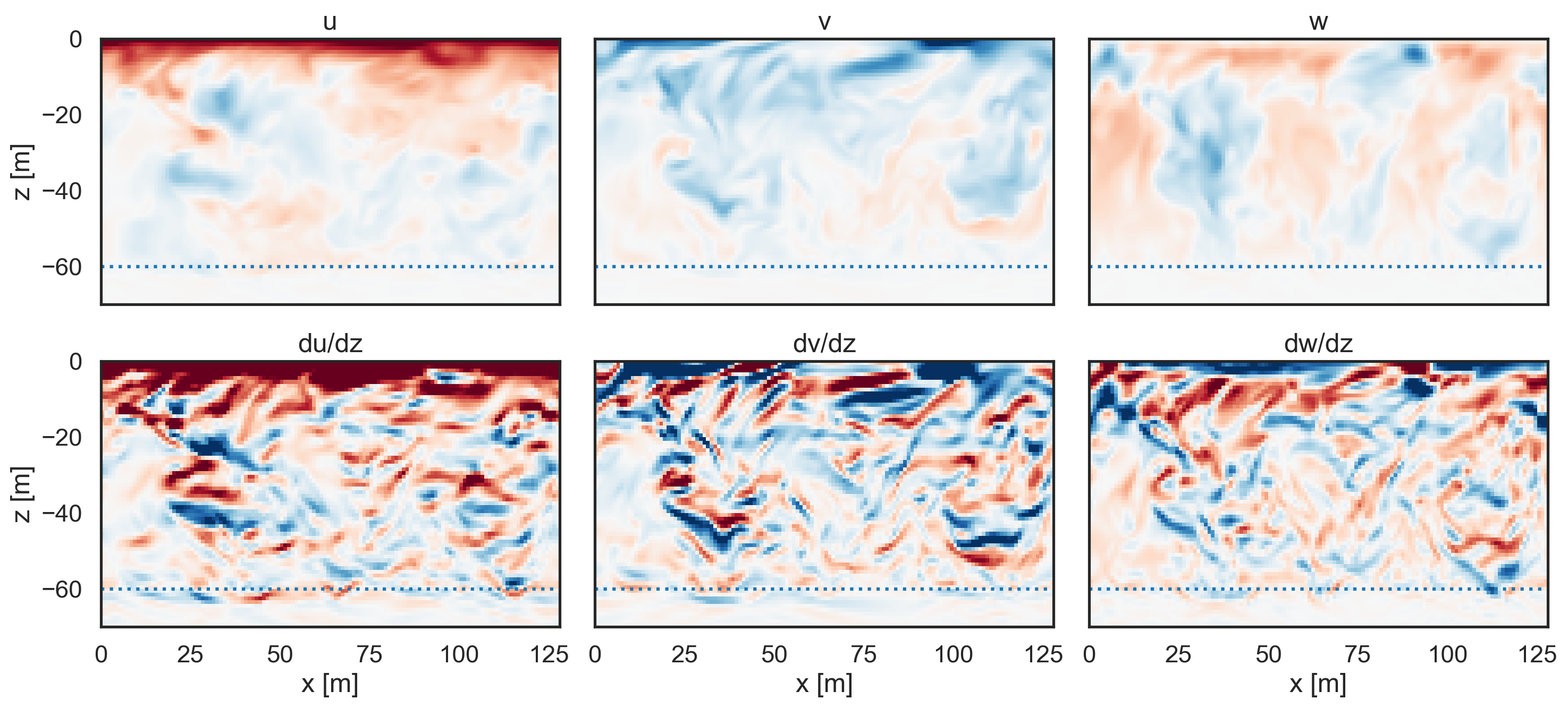
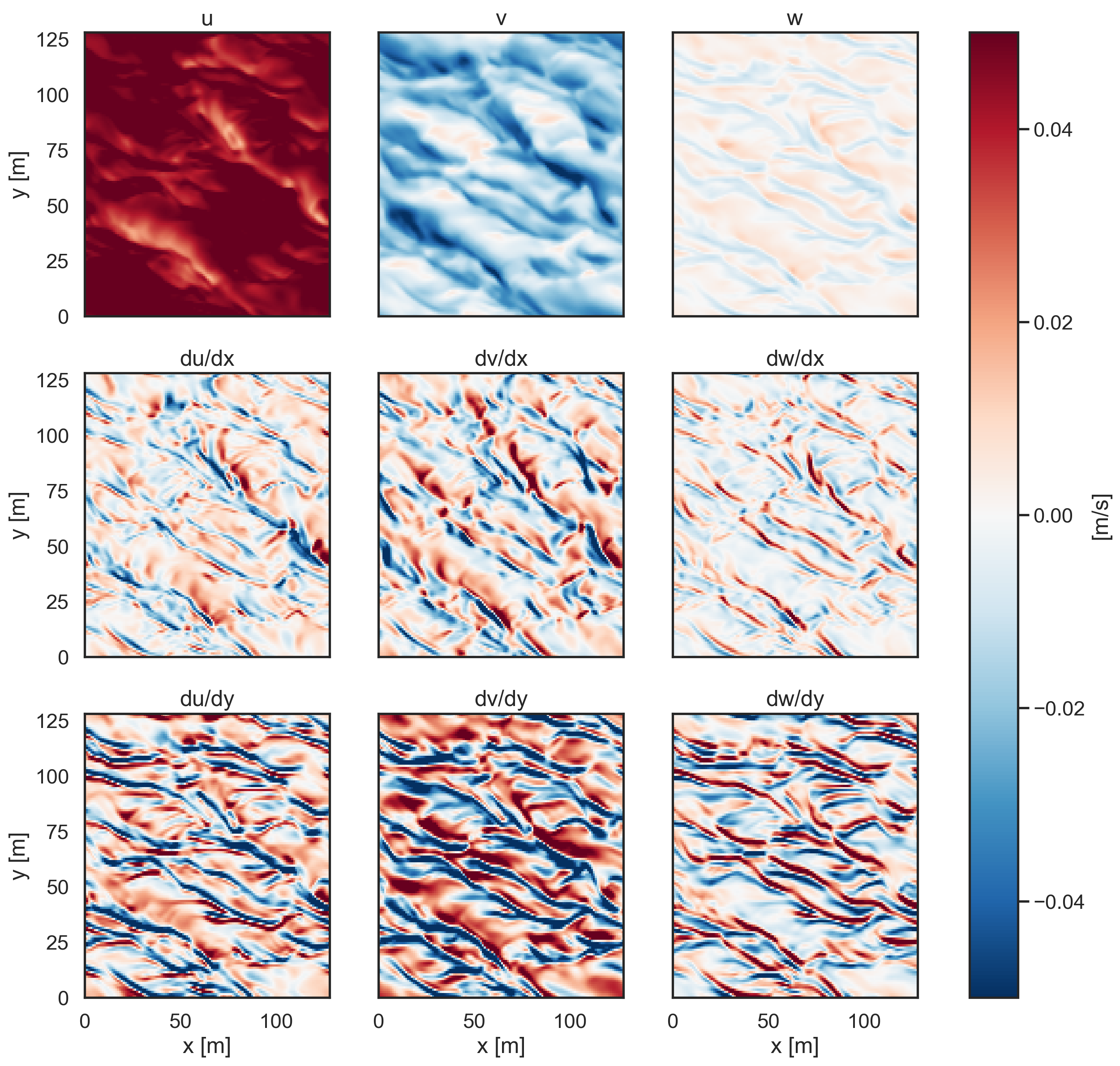
Visualize the velocity fields and gradients
[5]:
import matplotlib.pyplot as plt

fig, ax = plt.subplots(2, 3, figsize=(15, 7), sharey=True)

pc1 = ax[0, 0].pcolormesh(
    ds.xC, ds.zC, ds.u[:, 64, :], cmap="RdBu_r", vmin=-0.05, vmax=0.05
)
pc2 = ax[0, 1].pcolormesh(
    ds.xC, ds.zC, ds.v[:, 64, :], cmap="RdBu_r", vmin=-0.05, vmax=0.05
)
pc3 = ax[0, 2].pcolormesh(
    ds.xC, ds.zF, ds.w[:, 64, :], cmap="RdBu_r", vmin=-0.05, vmax=0.05
)
pc4 = ax[1, 0].pcolormesh(
    ds.xC, ds.zC, dudz[:, 64, :], cmap="RdBu_r", vmin=-0.005, vmax=0.005
)
pc5 = ax[1, 1].pcolormesh(
    ds.xC, ds.zC, dvdz[:, 64, :], cmap="RdBu_r", vmin=-0.005, vmax=0.005
)
pc6 = ax[1, 2].pcolormesh(
    ds.xC, ds.zF, dwdz[:, 64, :], cmap="RdBu_r", vmin=-0.005, vmax=0.005
)


ax[0, 0].plot([0, 128], [-60, -60], ":")
ax[0, 1].plot([0, 128], [-60, -60], ":")
ax[0, 2].plot([0, 128], [-60, -60], ":")
ax[1, 0].plot([0, 128], [-60, -60], ":")
ax[1, 1].plot([0, 128], [-60, -60], ":")
ax[1, 2].plot([0, 128], [-60, -60], ":")


ax[0, 0].set_ylabel("z [m]")
ax[1, 0].set_ylabel("z [m]")
ax[1, 0].set_xlabel("x [m]")
ax[1, 1].set_xlabel("x [m]")
ax[1, 2].set_xlabel("x [m]")

ax[0, 0].set_title("u")
ax[0, 1].set_title("v")
ax[0, 2].set_title("w")
ax[1, 0].set_title("du/dz")
ax[1, 1].set_title("dv/dz")
ax[1, 2].set_title("dw/dz")

ax[0, 0].set_xticks([]), ax[0, 1].set_xticks([]), ax[0, 2].set_xticks([])
ax[0, 0].set_ylim([-70, 0])

plt.tight_layout();

# cbar = fig.colorbar(pc1, ax=ax, orientation="vertical",label='[m/s]')
[6]:
fig, ax = plt.subplots(3, 3, figsize=(15, 14), sharey=True)

pc1 = ax[0, 0].pcolormesh(
    ds.xC, ds.yC, ds.u[-2, :, :], cmap="RdBu_r", vmin=-0.05, vmax=0.05
)
pc2 = ax[0, 1].pcolormesh(
    ds.xC, ds.yC, ds.v[-2, :, :], cmap="RdBu_r", vmin=-0.05, vmax=0.05
)
pc3 = ax[0, 2].pcolormesh(
    ds.xC, ds.yC, ds.w[-2, :, :], cmap="RdBu_r", vmin=-0.05, vmax=0.05
)
pc4 = ax[1, 0].pcolormesh(
    ds.xC, ds.yC, dudx[-2, :, :], cmap="RdBu_r", vmin=-0.005, vmax=0.005
)
pc5 = ax[1, 1].pcolormesh(
    ds.xC, ds.yC, dvdx[-2, :, :], cmap="RdBu_r", vmin=-0.005, vmax=0.005
)
pc6 = ax[1, 2].pcolormesh(
    ds.xC, ds.yC, dwdx[-2, :, :], cmap="RdBu_r", vmin=-0.005, vmax=0.005
)
pc7 = ax[2, 0].pcolormesh(
    ds.xC, ds.yC, dudy[-2, :, :], cmap="RdBu_r", vmin=-0.005, vmax=0.005
)
pc8 = ax[2, 1].pcolormesh(
    ds.xC, ds.yC, dvdy[-2, :, :], cmap="RdBu_r", vmin=-0.005, vmax=0.005
)
pc9 = ax[2, 2].pcolormesh(
    ds.xC, ds.yC, dwdy[-2, :, :], cmap="RdBu_r", vmin=-0.005, vmax=0.005
)


ax[0, 0].set_ylabel("y [m]")
ax[1, 0].set_ylabel("y [m]")
ax[2, 0].set_ylabel("y [m]")
ax[2, 0].set_xlabel("x [m]")
ax[2, 1].set_xlabel("x [m]")
ax[2, 2].set_xlabel("x [m]")

ax[0, 0].set_title("u")
ax[0, 1].set_title("v")
ax[0, 2].set_title("w")
ax[1, 0].set_title("du/dx")
ax[1, 1].set_title("dv/dx")
ax[1, 2].set_title("dw/dx")
ax[2, 0].set_title("du/dy")
ax[2, 1].set_title("dv/dy")
ax[2, 2].set_title("dw/dy")

ax[0, 0].set_xticks([]), ax[0, 1].set_xticks([]), ax[0, 2].set_xticks([])
ax[1, 0].set_xticks([]), ax[1, 1].set_xticks([]), ax[1, 2].set_xticks([])
cbar = fig.colorbar(pc1, ax=ax, orientation="vertical", label="[m/s]");
Calculate structure functions
After visualizing the three-dimensional velocity fields and their gradients, we are ready to calculate several different structure functions. We do this by calling the fluidsf.generate_structure_functions_3d module and feeding in the velocity fields, grid information, and desired structure functions. Note that we only use the upper 60 grid points (or meters) for this analysis, since we are interested in upper ocean boundary layer dynamics.
[7]:
import fluidsf

nn = 128

sf = fluidsf.generate_structure_functions_3d(
    ds.u.values[-60:, :, :],
    ds.v.values[-60:, :, :],
    ds.w.values[-60:, :, :],
    ds.xF.values[:],
    ds.yF.values[:],
    ds.zF.values[-60:],
    sf_type=["ASF_V", "LL", "LLL", "LTT"],
    boundary=["periodic-x", "periodic-y"],
)
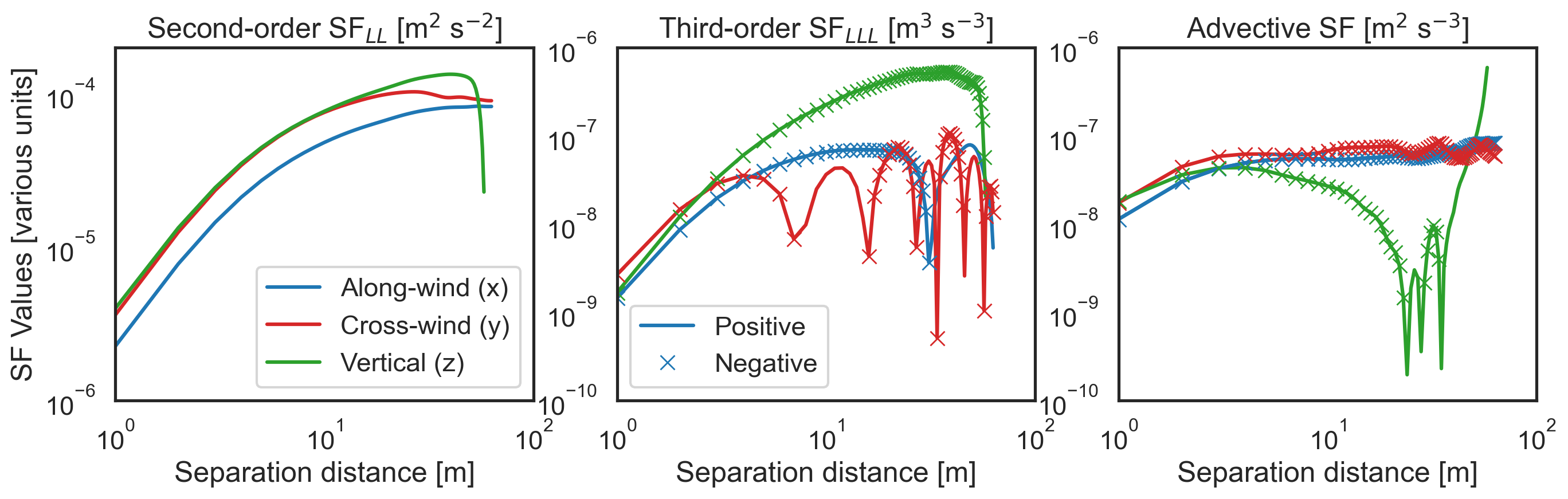
The package has now created a library of structure functions, with each structure function calculated using three different separation directions (x, y, or z). Below we plot the second- and third-order longitudinal structure functions, and the advective structure function, in each of these separation directions. Note that the longitudinal component of velocity varies with the separation direction (x\(\rightarrow\) u, y\(\rightarrow\) v, and
z\(\rightarrow\) w).
Plot structure function results
[8]:
fig, ax = plt.subplots(1, 3, figsize=(16, 4), sharey=False)

ax[0].loglog(
    sf["x-diffs"], abs(sf["SF_LL_x"]), color="tab:blue", label="Along-wind (x)"
)
ax[0].loglog(sf["y-diffs"], abs(sf["SF_LL_y"]), color="tab:red", label="Cross-wind (y)")
ax[0].loglog(sf["z-diffs"], abs(sf["SF_LL_z"]), color="tab:green", label="Vertical (z)")

ax[0].loglog(
    sf["x-diffs"], -(sf["SF_LL_x"]), color="tab:blue", marker="x", linestyle="None"
)
ax[0].loglog(
    sf["y-diffs"], -(sf["SF_LL_y"]), color="tab:red", marker="x", linestyle="None"
)
ax[0].loglog(
    sf["z-diffs"], -(sf["SF_LL_z"]), color="tab:green", marker="x", linestyle="None"
)

ax[0].set_xlabel("Separation distance [m]")
ax[0].set_title("Second-order SF$_{LL}$ [m$^2$ s$^{-2}$]")
ax[0].set_ylim([1e-6, 2e-4])
ax[0].set_xlim([1, 100])
ax[0].set_ylabel("SF Values [various units]")
ax[0].legend()
ax[1].loglog(sf["x-diffs"], abs(sf["SF_LLL_x"]), color="tab:blue", label="Positive")
ax[1].loglog(sf["y-diffs"], abs(sf["SF_LLL_y"]), color="tab:red")
ax[1].loglog(sf["z-diffs"], abs(sf["SF_LLL_z"]), color="tab:green")

ax[1].loglog(
    sf["x-diffs"],
    -(sf["SF_LLL_x"]),
    color="tab:blue",
    marker="x",
    linestyle="None",
    label="Negative",
)
ax[1].loglog(
    sf["y-diffs"], -(sf["SF_LLL_y"]), color="tab:red", marker="x", linestyle="None"
)
ax[1].loglog(
    sf["z-diffs"], -(sf["SF_LLL_z"]), color="tab:green", marker="x", linestyle="None"
)

ax[1].set_xlabel("Separation distance [m]")
ax[1].set_title("Third-order SF$_{LLL}$ [m$^3$ s$^{-3}$]")
ax[1].set_ylim([1e-10, 1e-6])
ax[1].set_xlim([1, 100])
ax[1].legend()
ax[2].loglog(
    sf["x-diffs"],
    abs(sf["SF_advection_velocity_x"]),
    color="tab:blue",
    label="Positive",
)
ax[2].loglog(sf["y-diffs"], abs(sf["SF_advection_velocity_y"]), color="tab:red")
ax[2].loglog(sf["z-diffs"], abs(sf["SF_advection_velocity_z"]), color="tab:green")

ax[2].loglog(
    sf["x-diffs"],
    -(sf["SF_advection_velocity_x"]),
    color="tab:blue",
    marker="x",
    label="Negative",
)
ax[2].loglog(
    sf["y-diffs"],
    -(sf["SF_advection_velocity_y"]),
    color="tab:red",
    marker="x",
    linestyle="None",
)
ax[2].loglog(
    sf["z-diffs"],
    -(sf["SF_advection_velocity_z"]),
    color="tab:green",
    marker="x",
    linestyle="None",
)

ax[2].set_xlabel("Separation distance [m]")
ax[2].set_title("Advective SF [m$^2$ s$^{-3}$]")
ax[2].set_ylim([1e-10, 1e-6])
ax[2].set_xlim([1, 100]);